What is a Geometric Random Variable?
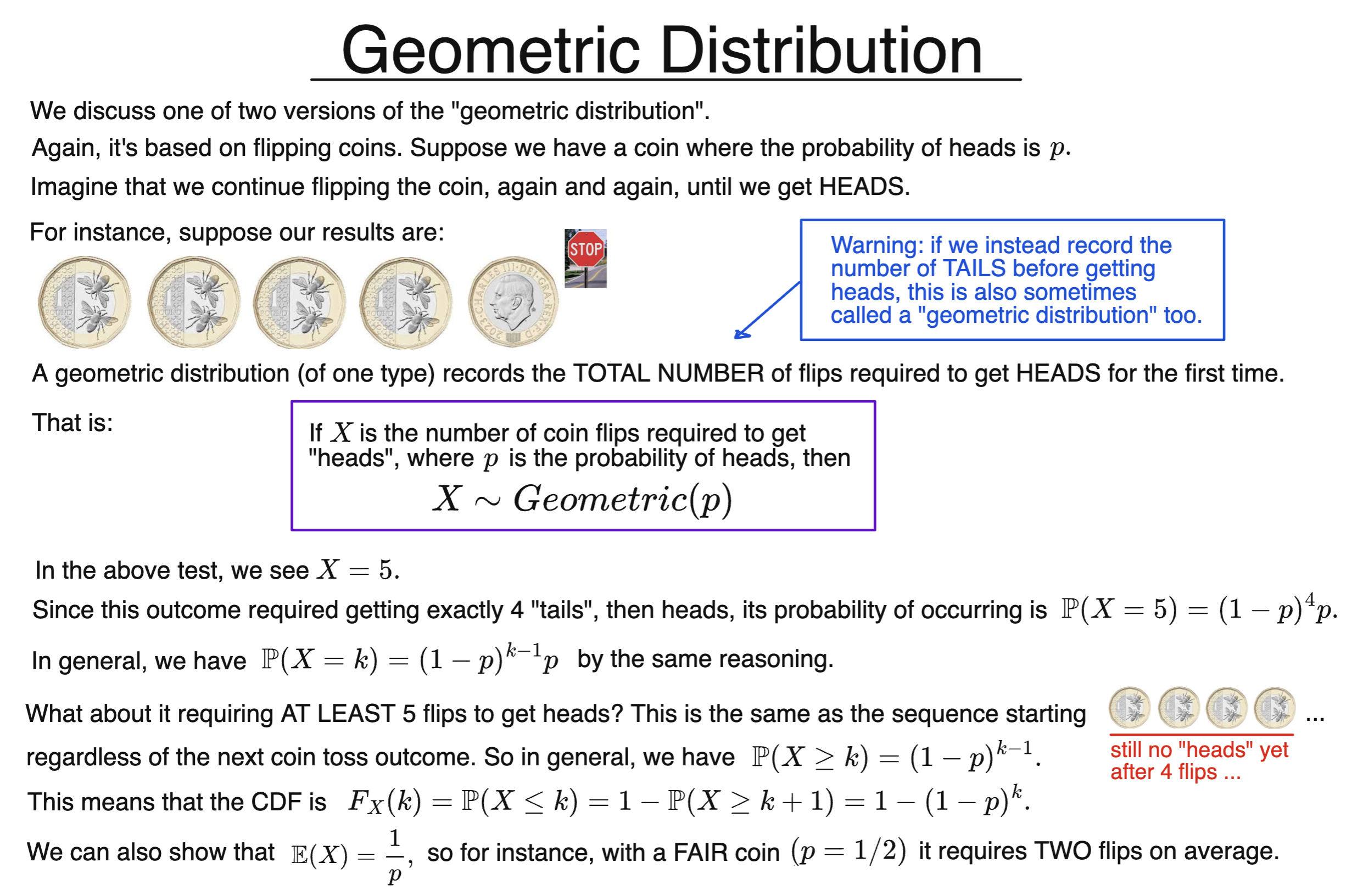
The geometric distribution arises when we continue running a series of identical trials, as many times as needed, to get a “success”.
Each trial must have exactly two outcomes, “success” or “failure”, like flipping a coin. If we think of getting “heads” as a success, we continue flipping the coin until that outcome is obtained.
The trials don’t have to involve flipping coins, but must be independent, with the same probability of success $p$ for each one.
A geometric random variable $X$ is then the number of trials needed to achieve one success (including the final, successful trial itself). We write:
$$X \sim \text{Geom}(p) $$
Alternatively, sometimes the geometric distribution is instead defined as the number of failures before the first success. You can recognise when someone is using this because the possible values will be $0,1,2, \dots $
| Notation: | $X \sim \text{Geom}(p)$ |
| Type: | $ \text{Discrete} $ |
| PMF: | $\mathbb{P}(X = k) = (1-p)^{k-1}p $ |
| Support: | $k \in \{1,2,3,\dots\}$ |
| Mean: | $\mathbb{E}(X) = 1/p$ |
| Variance: | $\mathbb{V}\text{ar}(X) = \frac{1-p}{p^2}$ |