What is a Joint PDF?
A joint PDF is a bit like a joint PMF, but for continuous random variables rather than discrete ones.
Very roughly, the value of the joint PDF at the point $X=x$ and $Y=y$ tells us how likely it is for X and Y to be “nearby” these points, respectively. Intuitively, we can think of it like a “relative probability”.
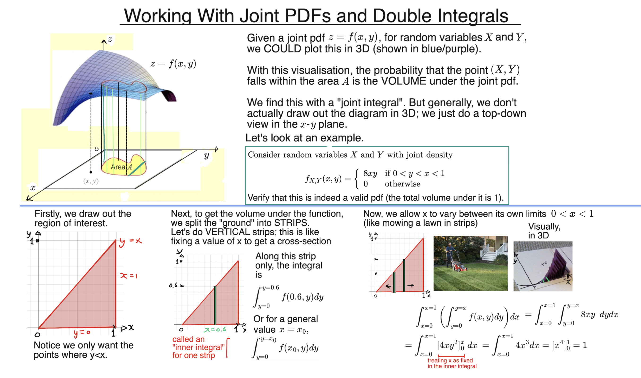
More carefully, to find the probability that X and Y lie within a certain region A in the x-y plane, we look at the volume under the PDF above that region (see diagram).
Since we find volumes by performing a double integral, this is what we need to do here too.
We complete a double integral by first fixing one variable, and then allowing the other variable to range over its appropriate limits. This maps out a “strip” in the x-y plane. We then repeat this process for all values of the first variable to “add up” all the strips.
We could also compute the example integral from the slide by first fixing a value of $y$ (a horizontal strip), and then letting $x$ vary between $y$ and $1$. That is, the integral can be written as:
$$ \int_{y=0}^{y=1} \int_{x=y}^{x=1} \ 8xy \ dxdy $$
We calculate this by first doing the “inner” integral, now treating $y$ as a constant here:
$$ = \int_ {y=0}^{y=1} \ \left[4x^2y \right]^{x=1}_{x=y} \ \ dy = \int _{y=0}^{y=1} \ 4y-4y^3 \ dy $$
Then, we do the outer integral over $y$:
$$ = \left[ 2y^2-y^4 \right]_{y=0}^{y=1} = (2-1)-(0-0)=1 $$
Since $X$ and $Y$ must end up somewhere, we always get 1 when we integrate the whole pdf $f_{X,Y}$ to give the total probability underneath it.