What is Covariance?
Roughly speaking, we say that two variables are “positively associated” if they tend to move together.
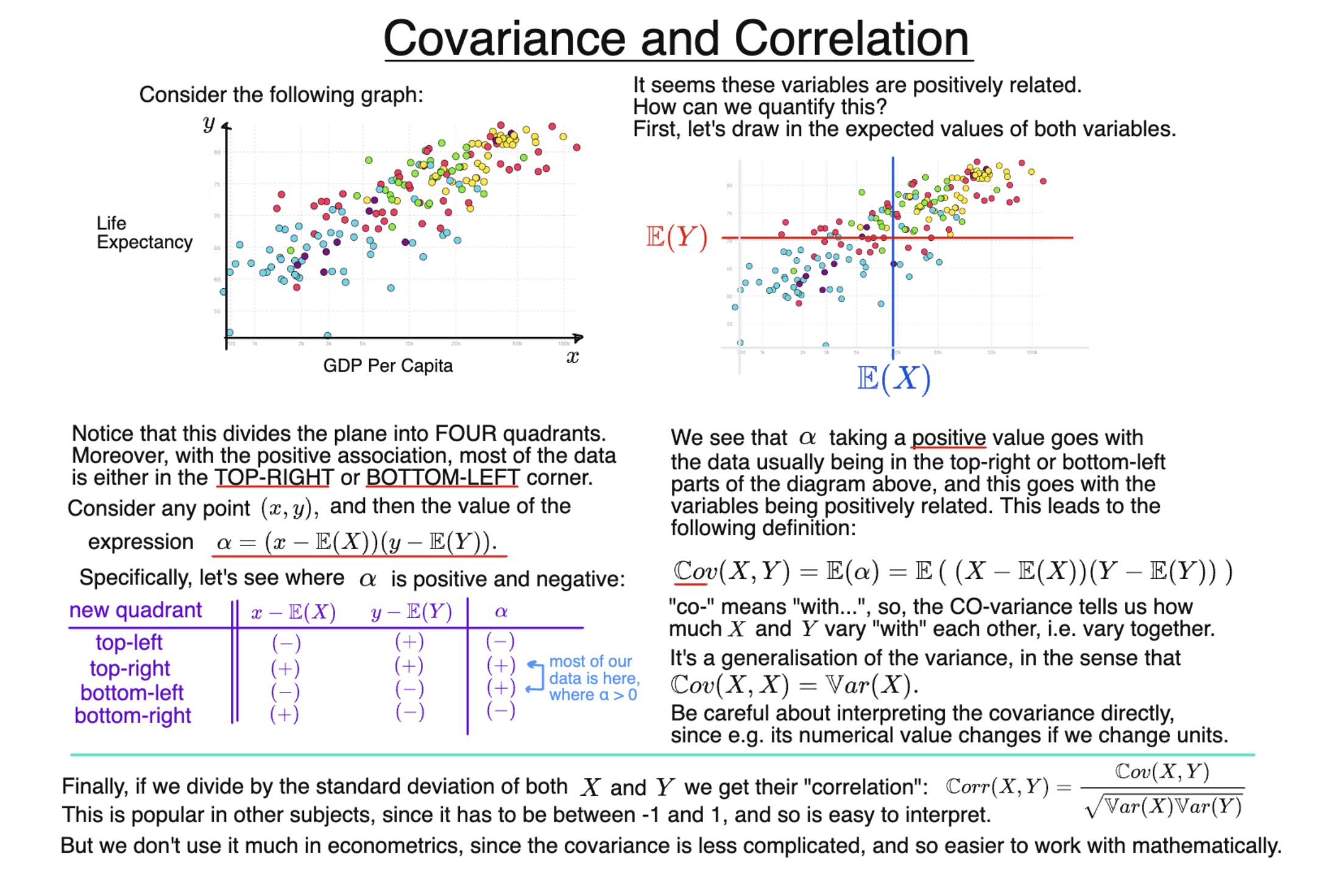
As a first step to formalising this, consider the case where $X$ and $Y$ are such that:
$$ \text{If } \ X - \mathbb{E}(X) \gt 0, \ \text{then typically } \ Y - \mathbb{E}(Y) \gt 0 $$
$$ \text{If } \ X - \mathbb{E}(X) \lt 0, \ \text{then typically } \ Y - \mathbb{E}(Y) \lt 0 $$
That is: if $X$ is greater than its own mean, then usually $Y$ will be as well; and conversely, if $X$ is less than its own mean, then $Y$ will tend to be less than its own mean too.
Then this implies that the following, random expression is usually positive:
$$ \left(X - \mathbb{E}(X) \right) \left( Y - \mathbb{E}(Y) \right) $$
Hence, we define the covariance of $X$ and $Y$ as its expectation:
$$ \mathbb{C}\text{ov}(X,Y) = \mathbb{E} \left( \left(X - \mathbb{E}(X) \right) \left( Y - \mathbb{E}(Y) \right) \right) $$
Intuitively, $ \mathbb{C}\text{ov}(X,Y) $ measures how much $X$ and $Y$ “vary together” (indeed, “co-” means “with-”).
If $X$ and $Y$ are independent, then $ \mathbb{C}\text{ov}(X,Y) =0$ (though the converse is not true). If they have a negative association, we instead have $ \mathbb{C}\text{ov}(X,Y) \lt 0$.
The covariance is a generalisation of the variance, in the sense that the covariance of a random variable with itself is precisely its variance:
$$ \mathbb{C}\text{ov}(X,X) = \mathbb{V}\text{ar}(X) $$
An equivalent expression for the covariance is:
$$ \mathbb{C}\text{ov}(X,Y) = \mathbb{E}(XY)-\mathbb{E} (X)\mathbb{E} (Y) $$
The numerical value of the covariance is hard to interpret, because it is sensitive to a choice of unit.
For instance, suppose we are interested in the covariance of GDP and life expectancy, as in the example in the slide. Suppose further that we decide to measure $X$ in thousands of dollars, rather than in dollars as shown. Then all of $X$, $\mathbb{E}(X)$, and $\mathbb{C}\text{ov}(X,Y)$ will get $1000$ times smaller; though of course, nothing substantial has changed about the relationship between $X$ and $Y$.
In general, we can expand out brackets in a natural way:
$$ \mathbb{C}\text{ov}(aX+b,Y) = a\ \mathbb{C}\text{ov}(X,Y) $$
since adding $b$ just shifts $X$, and so does not change the extent to which $X$ and $Y$ move together. We also have:
$$ \mathbb{C}\text{ov}(X_1+X_2,Y) = \mathbb{C}\text{ov}(X_1,Y) + \mathbb{C}\text{ov}(X_2,Y) $$
and similar rules for $Y$.
However, in econometrics, we are often just interested in the sign of the covariance, or whether or not it is equal to zero.
What is Correlation?
The correlation between $X$ and $Y$ is like its covariance, except scaled so that it must be between $-1$ and $1$. It is possible to show that this is achieved by taking the covariance and dividing by the standard deviation of both $X$ and $Y$. That is:
$$ \mathbb{C}\text{orr}(X,Y) \ = \ \frac{\mathbb{C}\text{ov}(X,Y)} { \sqrt{\mathbb{V}\text{ar}(X) \mathbb{V}\text{ar}(Y)}} $$
Although easier to interpret directly, the correlation is not often used directly in econometrics, because the covariance is easy to expand out, and in general much simpler to work with from a theory point of view.