What is the Mean Squared Error (MSE)?
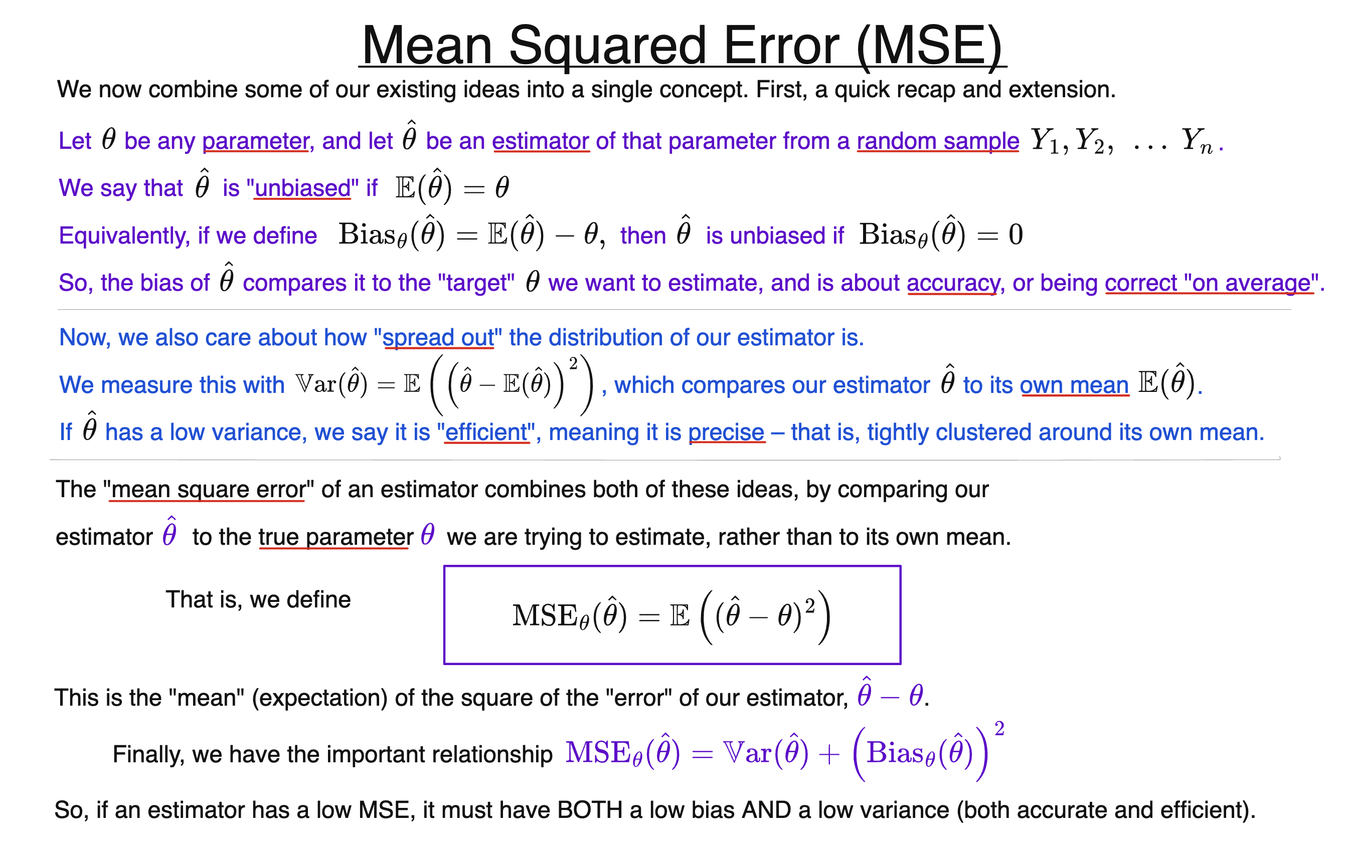
The mean-squared error of an estimator $\hat{\theta}$ of a parameter $\theta$ is the expectation of the square of its difference from $\theta$:
$$\operatorname{MSE}_{\theta}(\hat{\theta})= \mathbb{E} \left( (\hat{\theta}-\theta)^2 \right)$$
As usual, we square the error $\hat{\theta}-\theta$ to prevent positive and negative deviations from “cancelling out”.
If we define the bias of an estimator:
$$\operatorname{Bias}_{\theta}(\hat{\theta})=\mathbb{E}(\hat{\theta})-\theta$$
Then we also have the decomposition:
$$\operatorname{MSE}_ {\theta}(\hat{\theta}) = \left(\operatorname{Bias}_{\theta}(\hat{\theta}) \right)^2 + \mathbb{V}\text{ar}(\hat{\theta})$$
So, if the $\operatorname{MSE}$ is small, the estimator must have both a low bias and a low variance. That is, it must be both accurate and precise.
If the $\operatorname{MSE}$ of a sequence $\hat{\theta}_1, \hat{\theta}_2, \dots $ tends to $0$ as $n \to \infty$, then the sequence is consistent, but the converse is not true.