What is Convergence in Distribution?
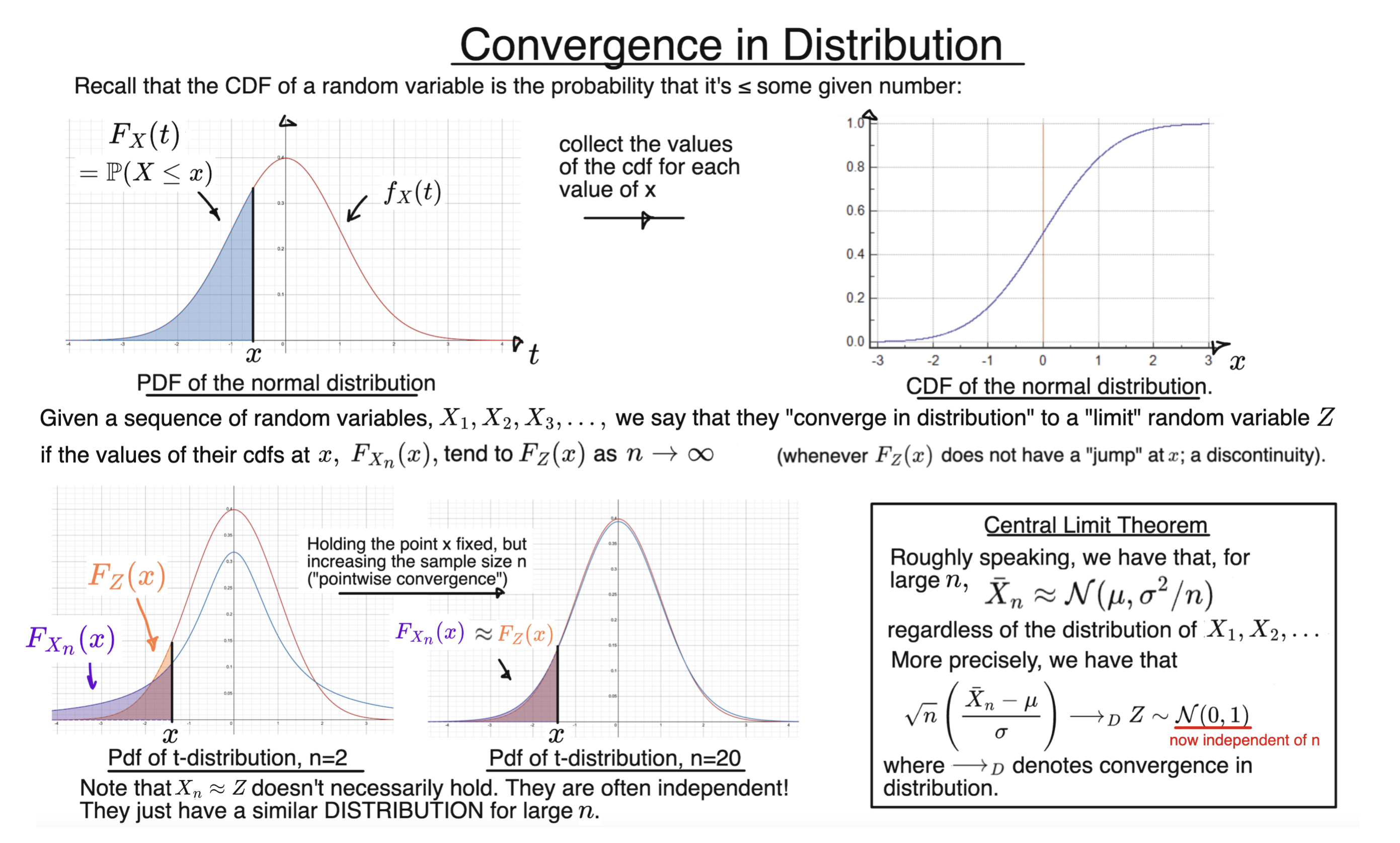
The definition of convergence in distribution for a sequence of random variables $X_1, X_2, X_3, \dots $ and a “limit” random variable $Z$ relates to the sequence of their CDFs, $F_{X_n}$, approaching the CDF of $Z$, as the term number $n$ tends to $\infty$.
We formalise this by first fixing the argument $x$ of the CDFs, and then saying that:
$$ \lim_{n \to \infty} F_{X_n}(x) = F_Z(x) $$
We also stipulate that the condition only needs to hold at points $x$ where the CDF of $Z$ is continuous.
This is closely related to the notion of “pointwise convergence”, since we are working with one value of $x$ at a time; fixing the value of $x$ first and then comparing the CDFs at that point. However, pointwise convergence does not make an exception at points of discontinuity. If the CDF of $Z$ is continuous, convergence in distribution is exactly the same as pointwise convergence of the CDFs.
Pointwise convergence contrasts with “uniform convergence”, where we would look at how far apart the entire CDFs are overall (focusing on the “worst case” for $x$).
If the sequence $X_1, X_2, X_3, … $ does tend in distribution to $Z$, we write
$$ X_n \overset{d}{\longrightarrow} Z $$
In the slide, we illustrate that a sequence of random variables, each with a $t$-distribution with $(n-1)$ degrees of freedom, converges to a standard normal random variable. This does not require these random variables to be independent.
On the other hand, we also have the central limit theorem.
Suppose now that $X_1, X_2, X_3, \dots $ are independent random variables, all with the same distribution, and with finite mean and variance $ \mathbb{E}(X_n) = \mu $ and $\mathbb{V}\text{ar}(X_n) = \sigma^2 $ for all $n$. In statistics, we call this a “random sample”.
Informally, if $ \bar{X}_n $ is the sample mean (average) of the first $n$, then for large $n$, it will be approximately true that:
$$ \bar{X}_n \sim \mathcal{N}(\mu, \sigma^2/n) $$
This is true regardless of the initial distribution – though the approximation is generally “better” the “closer to normal” the original sequence is.
To formalise this, we need to move the " $n $" in the last expression over to the left hand side, so there is a fixed “target” distribution to converge to. We typically move the $\mu$ and $\sigma^2$ over too, to get:
$$ \sqrt{n} \left( \frac{\bar{X}_n - \mu}{\sigma} \right) \overset{d}{\longrightarrow} Z, \ \ \ Z \sim \mathcal{N}(0,1)$$
We can also write $ \sqrt{n} \left( \frac{\bar{X}_n - \mu}{\sigma} \right) \overset{a}{\sim} \mathcal{N}(0,1) $ to say this is the “asymptotic” distribution of the sequence.
Note that saying that two random variables have a similar CDF, or even exactly the same CDF, is no guarantee that they will take similar values.
For instance, if we roll two fair dice, and let $X$ be the outcome of one, and $Y$ the outcome of the other. Then $X$ and $Y$ have exactly the same CDF, but are independent. That is, although the two dice tend to behave in the same way overall, they aren’t especially likely to come out close together.
This is the weakest of the three main notions of convergence, and is implied by the other two. We have:
$\text{Almost Sure Convergence} \Rightarrow \text{Convergence in Probability} \Rightarrow \text{Convergence in Distribution}$
However, if the “target” random variable $X$ happens to be a constant, then convergence in distribution is equivalent to convergence in probability.